Tutorial Advanced (Image Data Processing)

(Last updated: Feb 3, 2025)1

Here is an online version of this notebook in Google Colab. This online version is just for browsing. To work on this notebook, you need to copy a new one to your own Google Colab.

This tutorial covers image classification with PyTorch for a more complex dataset than the one used in the previous tutorial. More specifically, you will learn:

• How to identify overfitting.

• How to use data augmentation to palliate overfitting.

• How to carry out transfer learning to adapt a pretrained model to a different classification problem.

Warning

This tutorial notebook can take a long time to run due to the long training process.

import torch
import torchvision
import torch.nn as nn
import torch.optim as optim
import torchvision.transforms as transforms
from torchvision import models
from torchvision.utils import make_grid
from torch.utils.data import DataLoader, Subset
import numpy as np
import matplotlib.pyplot as plt
import copy

if torch.cuda.is_available():
    device = torch.device("cuda")          # use CUDA device
elif torch.backends.mps.is_available:
    device = torch.device("mps")          # use MPS device
else:
    device = torch.device("cpu")           # use CPU device
device

device(type='mps')

def set_seed(seed):
    """
    Seeds for reproducibility.

    Parameters
    ----------
    seed : int
        The seed.
    """
    np.random.seed(seed)
    torch.manual_seed(seed)
    if torch.cuda.is_available():
        torch.cuda.manual_seed(seed)
        torch.cuda.manual_seed_all(seed)
        torch.backends.cudnn.determinstic = True
        torch.backends.cudnn.benchmark = False
    elif torch.backends.mps.is_available():
        torch.mps.manual_seed(seed)

1. Preparation

Data

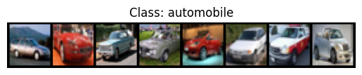
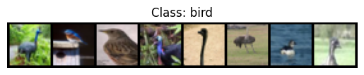
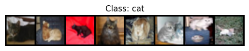
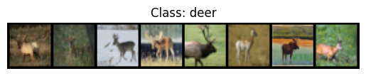
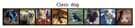
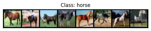
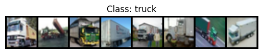
The CIFAR-10 dataset contains 60,000 32×32 RGB images evenly divided into 10 classes.

Let’s take a look at the dataset. The following cell load the data (downloading it on your ./data directory the first time):

cifar_10 = torchvision.datasets.CIFAR10(root="./data", train=True, download=True, transform=transforms.ToTensor())

Files already downloaded and verified

The images belong to one of these 10 classes:

classes = cifar_10.classes
print(classes)

['airplane', 'automobile', 'bird', 'cat', 'deer', 'dog', 'frog', 'horse', 'ship', 'truck']

Let’s display a bunch of images form each class:

for class_label, class_name in enumerate(classes):
    images = list()
    for image, label in cifar_10:
        if label == class_label:
            images.append(image)
            if len(images) >= 8:
                break
    plt.axis("off")
    plt.title("Class: " + class_name)
    plt.imshow(make_grid(images, nrow=8).permute(1, 2, 0))
    plt.show()

Now that we are familiar with the data, we can define the datasets and dataloaders:

# Define the transformation pipeline for the CIFAR-10 dataset
transform = transforms.Compose(
    [transforms.ToTensor(),
     transforms.Normalize((0.5, 0.5, 0.5), (0.5, 0.5, 0.5))])

# Load the CIFAR-10 training, validation and test datasets
dataset = torchvision.datasets.CIFAR10(root="./data", train=True, download=True, transform=transform)
train_dataset = Subset(dataset, range(0, 45000))
val_dataset = Subset(dataset, range(45000, 50000))
test_dataset = torchvision.datasets.CIFAR10(root="./data", train=False, download=True, transform=transform)

print(f"\nSize of training dataset: {len(train_dataset)}")
print(f"Size of validation dataset: {len(val_dataset)}")
print(f"Size of test dataset: {len(test_dataset)}")

Files already downloaded and verified
Files already downloaded and verified

Size of training dataset: 45000
Size of validation dataset: 5000
Size of test dataset: 10000

BATCH_SIZE = 64
train_dataloader = DataLoader(train_dataset, batch_size=BATCH_SIZE, shuffle=True)
val_dataloader = DataLoader(val_dataset, batch_size=BATCH_SIZE, shuffle=False)
test_dataloader = DataLoader(test_dataset, batch_size=BATCH_SIZE, shuffle=False)

Question for the reader: why do we shuffle the training data, but not the validation and test data?

Training

The training loop is similar to the one we used in the previous tutorial, with the following additions:

• We are using an ADAM optimizer. The difference with respect to SGD is that it does not use a static learning rate, but computes it dynamically based on estimates of the first as second moments. Intuitively, it takes into account how fast the gradients are changing to adapt the learning rate accordingly.

• At the end of each training epoch, we evaluate the model on:

  • The training dataset (exclusively for didactic purposes).

  • The validation dataset (to keep track of the best model along epochs).

Also, we define the function visualize_training to compare the evolution of the training and validation accuracies during the training.

def evaluate(model, dataloader):
    """
    Evaluate the model on the given dataloader.

    Parameters
    ----------
    model : torch.nn.Module
        The model to evaluate.
    dataloader : torch.utils.data.DataLoader
        DataLoader containing the evaluation dataset.

    Returns
    -------
    float
        The accuracy of the model on the evaluation dataset.
    """
    with torch.no_grad():
        correct = 0
        total = 0
        for images, labels in dataloader:
            images = images.to(device)
            labels = labels.to(device)

            outputs = model(images)
            predicted_labels = torch.argmax(outputs.data, 1)

            total += labels.size(0)
            correct += (predicted_labels == labels).sum().item()

    return correct / total


def train(model, train_dataloader, val_dataloader, n_epochs=50, lr=0.001, weight_decay=0.0001, compute_training_acc=True, verbose=False):
    """
    Train the given model.

    Parameters
    ----------
    model : torch.nn.Module
        The model to train.
    train_dataloader : torch.utils.data.DataLoader
        DataLoader containing the training dataset.
    val_dataloader : torch.utils.data.DataLoader
        DataLoader containing the validation dataset.
    n_epochs : int (optional)
        Number of epochs for training. Default is 50.
    lr : float (optional)
        Learning rate for training. Default is 0.001.
    weight_decay : float (optional)
        L2 regularization parameter
    compute_training_acc : bool (optional)
        Flag to compute training accuracy every epoch.
    print_batch_loss : bool (optional)
        Flag to print loss evolution inside batches.

    Returns
    -------
    tuple
        A tuple containing the best model, training losses, training accuracies, and validation accuracies.
    """
    train_losses = []
    train_accuracies = []
    val_accuracies = []
    max_val_acc = 0
    best_model = None

    criterion = nn.CrossEntropyLoss()
    optimizer = optim.Adam(model.parameters(), lr=lr, weight_decay=weight_decay)

    for epoch in range(n_epochs):
        epoch_losses = []
        model.train()

        for i, (images, labels) in enumerate(train_dataloader):
            images = images.to(device)
            labels = labels.to(device)

            optimizer.zero_grad()
            outputs = model(images)
            loss = criterion(outputs, labels)
            loss.backward()
            optimizer.step()

            epoch_losses.append(loss.item())

            if verbose and i % 100 == 0:
                print(f"Epoch {epoch} | Batch {i}/{len(train_dataloader)} | Training loss: {'{0:.4f}'.format(loss.item())}")

        train_loss = np.mean(epoch_losses).item()
        train_losses.append(train_loss)

        val_acc = evaluate(model, val_dataloader)
        val_accuracies.append(val_acc)

        if (val_acc > max_val_acc):
            max_val_acc = val_acc
            best_model = copy.deepcopy(model)

        if compute_training_acc:
            train_acc = evaluate(model, train_dataloader)
            train_accuracies.append(train_acc)
            print(f"Epoch {epoch} | Training loss: {'{0:.4f}'.format(train_loss)} | Training accuracy: {'{0:.4f}'.format(train_acc)} | Validation accuracy: {'{0:.4f}'.format(val_acc)}")

        else:
            print(f"Epoch {epoch} | Training loss: {'{0:.4f}'.format(train_loss)} | Validation accuracy: {'{0:.4f}'.format(val_acc)}")

    return best_model, train_losses, train_accuracies, val_accuracies


def visualize_training(train_accuracies, val_accuracies):
    """
    Visualize the training process.

    Parameters
    ----------
    train_accuracies : list)
        List of training accuracies.
    val_accuracies : list)
        List of validation accuracies.
    """
    plt.title("Training evolution")
    plt.xlabel("Epoch")
    plt.ylabel("Accuracy")
    plt.gca().set_ylim(0, 1)
    epochs = range(1, len(train_accuracies) + 1)
    plt.plot(epochs, train_accuracies, label="Training")
    plt.plot(epochs, val_accuracies, label="Validation")
    plt.legend(loc="lower right")
    plt.show()

2. Using a simple CNN

We define a simple CNN model to classify this data into the 10 different classes:

class ConvNet(nn.Module):
    def __init__(self, n_classes):
        super(ConvNet, self).__init__()
        self.conv_layers = nn.Sequential(
            nn.Conv2d(3, 32, kernel_size=3, padding=1),  # Conv layer with 32 filters of size 3x3
            nn.ReLU(),  # ReLU activation
            nn.MaxPool2d(kernel_size=2, stride=2),  # Max pooling layer with pool size 2x2
            nn.Conv2d(32, 64, kernel_size=5),  # Conv layer with 64 filters of size 5x5
            nn.ReLU(),  # ReLU activation
            nn.MaxPool2d(kernel_size=3, stride=3),  # Max pooling layer with pool size 3x3
            nn.Conv2d(64, 64, kernel_size=3),  # Conv layer with 64 filters of size 3x3
            nn.ReLU()  # ReLU activation
        )
        self.fc_layers = nn.Sequential(
            nn.Flatten(),  # Flatten layer
            nn.Linear(64 * 2 * 2, 64),  # Fully connected layer
            nn.ReLU(),  # ReLU activation
            nn.Linear(64, n_classes)  # Output layer
        )

    def forward(self, x):
        x = self.conv_layers(x)
        x = self.fc_layers(x)
        return x

Now, we can train the model using our train function.

set_seed(42) # Seed for reproducibility of the results
model = ConvNet(n_classes=10)
model = model.to(device)
model_simplenet, train_losses, train_accuracies, val_accuracies = train(model, train_dataloader, val_dataloader)

Epoch 0 | Training loss: 1.5863 | Training accuracy: 0.5050 | Validation accuracy: 0.5052
Epoch 1 | Training loss: 1.2678 | Training accuracy: 0.5865 | Validation accuracy: 0.5876
Epoch 2 | Training loss: 1.1085 | Training accuracy: 0.6411 | Validation accuracy: 0.6292
Epoch 3 | Training loss: 0.9957 | Training accuracy: 0.6867 | Validation accuracy: 0.6694
Epoch 4 | Training loss: 0.9088 | Training accuracy: 0.6932 | Validation accuracy: 0.6658
Epoch 5 | Training loss: 0.8440 | Training accuracy: 0.7282 | Validation accuracy: 0.6900
Epoch 6 | Training loss: 0.7869 | Training accuracy: 0.7183 | Validation accuracy: 0.6754
Epoch 7 | Training loss: 0.7421 | Training accuracy: 0.7674 | Validation accuracy: 0.7136
Epoch 8 | Training loss: 0.6953 | Training accuracy: 0.7710 | Validation accuracy: 0.7152
Epoch 9 | Training loss: 0.6614 | Training accuracy: 0.7858 | Validation accuracy: 0.7176
Epoch 10 | Training loss: 0.6239 | Training accuracy: 0.7987 | Validation accuracy: 0.7316
Epoch 11 | Training loss: 0.5968 | Training accuracy: 0.8139 | Validation accuracy: 0.7244
Epoch 12 | Training loss: 0.5707 | Training accuracy: 0.8191 | Validation accuracy: 0.7284
Epoch 13 | Training loss: 0.5478 | Training accuracy: 0.8321 | Validation accuracy: 0.7310
Epoch 14 | Training loss: 0.5221 | Training accuracy: 0.8368 | Validation accuracy: 0.7306
Epoch 15 | Training loss: 0.5094 | Training accuracy: 0.8393 | Validation accuracy: 0.7316
Epoch 16 | Training loss: 0.4808 | Training accuracy: 0.8557 | Validation accuracy: 0.7338
Epoch 17 | Training loss: 0.4623 | Training accuracy: 0.8461 | Validation accuracy: 0.7270
Epoch 18 | Training loss: 0.4466 | Training accuracy: 0.8690 | Validation accuracy: 0.7348
Epoch 19 | Training loss: 0.4271 | Training accuracy: 0.8686 | Validation accuracy: 0.7278
Epoch 20 | Training loss: 0.4161 | Training accuracy: 0.8646 | Validation accuracy: 0.7228
Epoch 21 | Training loss: 0.3969 | Training accuracy: 0.8840 | Validation accuracy: 0.7298
Epoch 22 | Training loss: 0.3778 | Training accuracy: 0.8832 | Validation accuracy: 0.7294
Epoch 23 | Training loss: 0.3634 | Training accuracy: 0.8925 | Validation accuracy: 0.7300
Epoch 24 | Training loss: 0.3467 | Training accuracy: 0.8688 | Validation accuracy: 0.7132
Epoch 25 | Training loss: 0.3374 | Training accuracy: 0.8786 | Validation accuracy: 0.7118
Epoch 26 | Training loss: 0.3234 | Training accuracy: 0.9126 | Validation accuracy: 0.7344
Epoch 27 | Training loss: 0.3158 | Training accuracy: 0.9094 | Validation accuracy: 0.7300
Epoch 28 | Training loss: 0.2979 | Training accuracy: 0.9056 | Validation accuracy: 0.7246
Epoch 29 | Training loss: 0.2847 | Training accuracy: 0.9176 | Validation accuracy: 0.7276
Epoch 30 | Training loss: 0.2808 | Training accuracy: 0.9169 | Validation accuracy: 0.7252
Epoch 31 | Training loss: 0.2658 | Training accuracy: 0.9197 | Validation accuracy: 0.7240
Epoch 32 | Training loss: 0.2565 | Training accuracy: 0.9325 | Validation accuracy: 0.7216
Epoch 33 | Training loss: 0.2479 | Training accuracy: 0.9235 | Validation accuracy: 0.7262
Epoch 34 | Training loss: 0.2413 | Training accuracy: 0.9273 | Validation accuracy: 0.7168
Epoch 35 | Training loss: 0.2374 | Training accuracy: 0.9311 | Validation accuracy: 0.7174
Epoch 36 | Training loss: 0.2164 | Training accuracy: 0.9371 | Validation accuracy: 0.7280
Epoch 37 | Training loss: 0.2124 | Training accuracy: 0.9312 | Validation accuracy: 0.7236
Epoch 38 | Training loss: 0.2062 | Training accuracy: 0.9277 | Validation accuracy: 0.7156
Epoch 39 | Training loss: 0.2059 | Training accuracy: 0.9427 | Validation accuracy: 0.7180
Epoch 40 | Training loss: 0.1880 | Training accuracy: 0.9317 | Validation accuracy: 0.7104
Epoch 41 | Training loss: 0.1910 | Training accuracy: 0.9489 | Validation accuracy: 0.7186
Epoch 42 | Training loss: 0.1864 | Training accuracy: 0.9401 | Validation accuracy: 0.7138
Epoch 43 | Training loss: 0.1747 | Training accuracy: 0.9332 | Validation accuracy: 0.7162
Epoch 44 | Training loss: 0.1707 | Training accuracy: 0.9582 | Validation accuracy: 0.7184
Epoch 45 | Training loss: 0.1739 | Training accuracy: 0.9551 | Validation accuracy: 0.7148
Epoch 46 | Training loss: 0.1631 | Training accuracy: 0.9483 | Validation accuracy: 0.7190
Epoch 47 | Training loss: 0.1519 | Training accuracy: 0.9540 | Validation accuracy: 0.7220
Epoch 48 | Training loss: 0.1639 | Training accuracy: 0.9491 | Validation accuracy: 0.7122
Epoch 49 | Training loss: 0.1534 | Training accuracy: 0.9463 | Validation accuracy: 0.7190

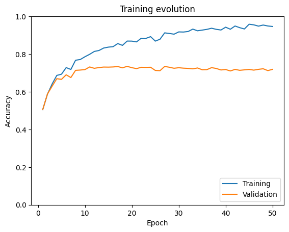
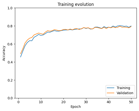
visualize_training(train_accuracies, val_accuracies)

print("Test accuracy: " + str(evaluate(model_simplenet, test_dataloader)))

Test accuracy: 0.7248

We observe that the model achieves a validation accuracy of 72% in 10 epochs. Beyond that, the training accuracy continues increasing, reaching almost perfect performance, but the validation accuracy stays constant with some fluctuations. This is an indicator of overfitting: the model is learning the training data very well, but it is not able to generalize to other data samples.

3. Data Augmentation

Data augmentation is a technique used to artificially increase the size and diversity of a training dataset. In the particular case of image classification, we can achieve this by applying transformations to the available images, such as rotating, flipping, cropping… This helps the classifier generalize better on data outside the training dataset, reducing overfitting.

image = cifar_10[7][0]
rotator = transforms.RandomRotation(degrees=(0,180))
flipper = transforms.RandomHorizontalFlip(p=1)
color_jitter = transforms.ColorJitter(brightness=.5, hue=.3)

# Visualize augmented images
plt.axis("off")
plt.imshow(make_grid([image, rotator(image), flipper(image), color_jitter(image)], nrow=4).permute(1, 2, 0))

<matplotlib.image.AxesImage at 0x13ff39e20>

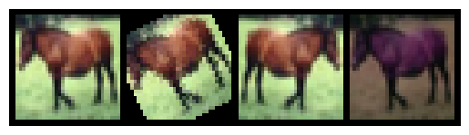
In this case, for example, using augmentations of that horse will allow the model to identify horses not only if they are similar to the training images, but also if they appear in different positions or under different light conditions.

Let’s add some augmentations to our training dataset. For that purpose, we need to include the augmentations in the transform pipeline:

# Define new transformation pipeline for the training dataset, including augmentations
transform_augmented = transforms.Compose([
    transforms.RandomHorizontalFlip(p=0.5),
    transforms.RandomCrop(32, padding=4),
    transforms.ToTensor(),
    transforms.Normalize((0.5, 0.5, 0.5), (0.5, 0.5, 0.5))])

# Redefine training dataset and dataloader
train_dataset_augmented = Subset(torchvision.datasets.CIFAR10(root="./data", train=True, download=True, transform=transform_augmented), range(0, 45000))
train_dataloader_augmented = DataLoader(train_dataset_augmented, batch_size=64, shuffle=True)

Files already downloaded and verified

Let’s train the model using the augmented dataset.

set_seed(42) # Seed for reproducibility of the results
model = ConvNet(n_classes=10)
model = model.to(device)
model_simplenet_augmented, train_losses, train_accuracies, val_accuracies = train(model, train_dataloader_augmented, val_dataloader)

Epoch 0 | Training loss: 1.6935 | Training accuracy: 0.4552 | Validation accuracy: 0.4910
Epoch 1 | Training loss: 1.3794 | Training accuracy: 0.5197 | Validation accuracy: 0.5454
Epoch 2 | Training loss: 1.2332 | Training accuracy: 0.5795 | Validation accuracy: 0.6102
Epoch 3 | Training loss: 1.1406 | Training accuracy: 0.6158 | Validation accuracy: 0.6428
Epoch 4 | Training loss: 1.0649 | Training accuracy: 0.6358 | Validation accuracy: 0.6632
Epoch 5 | Training loss: 1.0160 | Training accuracy: 0.6345 | Validation accuracy: 0.6714
Epoch 6 | Training loss: 0.9692 | Training accuracy: 0.6736 | Validation accuracy: 0.7002
Epoch 7 | Training loss: 0.9282 | Training accuracy: 0.6875 | Validation accuracy: 0.7104
Epoch 8 | Training loss: 0.8882 | Training accuracy: 0.7051 | Validation accuracy: 0.7204
Epoch 9 | Training loss: 0.8696 | Training accuracy: 0.6946 | Validation accuracy: 0.7138
Epoch 10 | Training loss: 0.8457 | Training accuracy: 0.6989 | Validation accuracy: 0.7072
Epoch 11 | Training loss: 0.8271 | Training accuracy: 0.7141 | Validation accuracy: 0.7302
Epoch 12 | Training loss: 0.8026 | Training accuracy: 0.7311 | Validation accuracy: 0.7470
Epoch 13 | Training loss: 0.7926 | Training accuracy: 0.7289 | Validation accuracy: 0.7410
Epoch 14 | Training loss: 0.7765 | Training accuracy: 0.7396 | Validation accuracy: 0.7462
Epoch 15 | Training loss: 0.7651 | Training accuracy: 0.7474 | Validation accuracy: 0.7580
Epoch 16 | Training loss: 0.7525 | Training accuracy: 0.7413 | Validation accuracy: 0.7530
Epoch 17 | Training loss: 0.7468 | Training accuracy: 0.7412 | Validation accuracy: 0.7466
Epoch 18 | Training loss: 0.7342 | Training accuracy: 0.7471 | Validation accuracy: 0.7494
Epoch 19 | Training loss: 0.7271 | Training accuracy: 0.7522 | Validation accuracy: 0.7596
Epoch 20 | Training loss: 0.7077 | Training accuracy: 0.7542 | Validation accuracy: 0.7612
Epoch 21 | Training loss: 0.7050 | Training accuracy: 0.7548 | Validation accuracy: 0.7548
Epoch 22 | Training loss: 0.7003 | Training accuracy: 0.7590 | Validation accuracy: 0.7650
Epoch 23 | Training loss: 0.6939 | Training accuracy: 0.7549 | Validation accuracy: 0.7564
Epoch 24 | Training loss: 0.6891 | Training accuracy: 0.7612 | Validation accuracy: 0.7676
Epoch 25 | Training loss: 0.6924 | Training accuracy: 0.7638 | Validation accuracy: 0.7694
Epoch 26 | Training loss: 0.6773 | Training accuracy: 0.7664 | Validation accuracy: 0.7590
Epoch 27 | Training loss: 0.6657 | Training accuracy: 0.7663 | Validation accuracy: 0.7688
Epoch 28 | Training loss: 0.6655 | Training accuracy: 0.7804 | Validation accuracy: 0.7812
Epoch 29 | Training loss: 0.6623 | Training accuracy: 0.7714 | Validation accuracy: 0.7750
Epoch 30 | Training loss: 0.6541 | Training accuracy: 0.7779 | Validation accuracy: 0.7794
Epoch 31 | Training loss: 0.6557 | Training accuracy: 0.7641 | Validation accuracy: 0.7676
Epoch 32 | Training loss: 0.6518 | Training accuracy: 0.7669 | Validation accuracy: 0.7662
Epoch 33 | Training loss: 0.6423 | Training accuracy: 0.7861 | Validation accuracy: 0.7830
Epoch 34 | Training loss: 0.6355 | Training accuracy: 0.7873 | Validation accuracy: 0.7818
Epoch 35 | Training loss: 0.6282 | Training accuracy: 0.7804 | Validation accuracy: 0.7754
Epoch 36 | Training loss: 0.6291 | Training accuracy: 0.7718 | Validation accuracy: 0.7698
Epoch 37 | Training loss: 0.6271 | Training accuracy: 0.7920 | Validation accuracy: 0.7844
Epoch 38 | Training loss: 0.6218 | Training accuracy: 0.7806 | Validation accuracy: 0.7698
Epoch 39 | Training loss: 0.6166 | Training accuracy: 0.7857 | Validation accuracy: 0.7848
Epoch 40 | Training loss: 0.6127 | Training accuracy: 0.7809 | Validation accuracy: 0.7782
Epoch 41 | Training loss: 0.6105 | Training accuracy: 0.7984 | Validation accuracy: 0.7888
Epoch 42 | Training loss: 0.6078 | Training accuracy: 0.7872 | Validation accuracy: 0.7806
Epoch 43 | Training loss: 0.6112 | Training accuracy: 0.7988 | Validation accuracy: 0.7836
Epoch 44 | Training loss: 0.6033 | Training accuracy: 0.8017 | Validation accuracy: 0.7966
Epoch 45 | Training loss: 0.6026 | Training accuracy: 0.7996 | Validation accuracy: 0.7850
Epoch 46 | Training loss: 0.6050 | Training accuracy: 0.7946 | Validation accuracy: 0.7864
Epoch 47 | Training loss: 0.5990 | Training accuracy: 0.7975 | Validation accuracy: 0.7836
Epoch 48 | Training loss: 0.5940 | Training accuracy: 0.7841 | Validation accuracy: 0.7790
Epoch 49 | Training loss: 0.5977 | Training accuracy: 0.7988 | Validation accuracy: 0.7912

visualize_training(train_accuracies, val_accuracies)

print("Test accuracy for agumented model: " + str(evaluate(model_simplenet_augmented, test_dataloader)))

Test accuracy for agumented model: 0.7844

We observe how, in this case, both training and validation accuracies evolve in a similar way, getting a higher accuracy in the validation and test datasets than in the previous experiment.

Feel free to experiment with more augmentation techniques, like random fips or crops. You can check more examples of augmentations in PyTorch here. Which augmentation types lead to the highest increase in performance for this dataset?

Also, try to reflect on how we have implemented data augmentation by answering the following questions:

• Inside a batch, we do not preserve the original version of the augmented images. In other words, augmented images are not copies of the original images, but we are just modifying the original images themselves. Why is this not a problem?

• Why are we adding augmentations only to the training dataset?

4. Transfer learning

Another way of improving performance is using a more complex architecture. Nevertheless, we probably do not have the computational resources needed to train such complex models.

An alternative to palliate this issue is, instead of training a whole model form scratch, taking advantage of an already pretrained model. Obviously, we cannot use a model that has been trained on a different dataset in an off-the-shelf manner, but the features captured by the intermediate layers can be leveraged for our taks.

We will use VGG19, a deep convolutional model trained on images of 1000 different classes from the ImageNet dataset.

First, let’s load the model and analyze its architecture:

model_vgg19 = models.vgg19(weights=models.VGG19_Weights.IMAGENET1K_V1)
model_vgg19

VGG(
  (features): Sequential(
    (0): Conv2d(3, 64, kernel_size=(3, 3), stride=(1, 1), padding=(1, 1))
    (1): ReLU(inplace=True)
    (2): Conv2d(64, 64, kernel_size=(3, 3), stride=(1, 1), padding=(1, 1))
    (3): ReLU(inplace=True)
    (4): MaxPool2d(kernel_size=2, stride=2, padding=0, dilation=1, ceil_mode=False)
    (5): Conv2d(64, 128, kernel_size=(3, 3), stride=(1, 1), padding=(1, 1))
    (6): ReLU(inplace=True)
    (7): Conv2d(128, 128, kernel_size=(3, 3), stride=(1, 1), padding=(1, 1))
    (8): ReLU(inplace=True)
    (9): MaxPool2d(kernel_size=2, stride=2, padding=0, dilation=1, ceil_mode=False)
    (10): Conv2d(128, 256, kernel_size=(3, 3), stride=(1, 1), padding=(1, 1))
    (11): ReLU(inplace=True)
    (12): Conv2d(256, 256, kernel_size=(3, 3), stride=(1, 1), padding=(1, 1))
    (13): ReLU(inplace=True)
    (14): Conv2d(256, 256, kernel_size=(3, 3), stride=(1, 1), padding=(1, 1))
    (15): ReLU(inplace=True)
    (16): Conv2d(256, 256, kernel_size=(3, 3), stride=(1, 1), padding=(1, 1))
    (17): ReLU(inplace=True)
    (18): MaxPool2d(kernel_size=2, stride=2, padding=0, dilation=1, ceil_mode=False)
    (19): Conv2d(256, 512, kernel_size=(3, 3), stride=(1, 1), padding=(1, 1))
    (20): ReLU(inplace=True)
    (21): Conv2d(512, 512, kernel_size=(3, 3), stride=(1, 1), padding=(1, 1))
    (22): ReLU(inplace=True)
    (23): Conv2d(512, 512, kernel_size=(3, 3), stride=(1, 1), padding=(1, 1))
    (24): ReLU(inplace=True)
    (25): Conv2d(512, 512, kernel_size=(3, 3), stride=(1, 1), padding=(1, 1))
    (26): ReLU(inplace=True)
    (27): MaxPool2d(kernel_size=2, stride=2, padding=0, dilation=1, ceil_mode=False)
    (28): Conv2d(512, 512, kernel_size=(3, 3), stride=(1, 1), padding=(1, 1))
    (29): ReLU(inplace=True)
    (30): Conv2d(512, 512, kernel_size=(3, 3), stride=(1, 1), padding=(1, 1))
    (31): ReLU(inplace=True)
    (32): Conv2d(512, 512, kernel_size=(3, 3), stride=(1, 1), padding=(1, 1))
    (33): ReLU(inplace=True)
    (34): Conv2d(512, 512, kernel_size=(3, 3), stride=(1, 1), padding=(1, 1))
    (35): ReLU(inplace=True)
    (36): MaxPool2d(kernel_size=2, stride=2, padding=0, dilation=1, ceil_mode=False)
  )
  (avgpool): AdaptiveAvgPool2d(output_size=(7, 7))
  (classifier): Sequential(
    (0): Linear(in_features=25088, out_features=4096, bias=True)
    (1): ReLU(inplace=True)
    (2): Dropout(p=0.5, inplace=False)
    (3): Linear(in_features=4096, out_features=4096, bias=True)
    (4): ReLU(inplace=True)
    (5): Dropout(p=0.5, inplace=False)
    (6): Linear(in_features=4096, out_features=1000, bias=True)
  )
)

The architecture is divided in two main modules:

• features: convolutional module that extracts features from the images. We will freeze this part, i.e. the parameters of these layers will not be modified in the optimization step.

• classifier: linear module that maps the features to the logits for each of the 1000 classes of the original model. We will change the linear layers of this module to adapt it to our output size (10, which is the number of classes in CIFAR10).

Question for the reader: what does the “19” on the model name stand for?.

The following code cell freezes/redefines the above mentioned modules:

# Freeze all parameters:
for param in model_vgg19.parameters():
    param.requires_grad = False

# Redefine linear layers in the classifier module (by redefining them, requires grad will be set to True by default)
model_vgg19.classifier[3] = nn.Linear(4096, 512)
model_vgg19.classifier[6] = nn.Linear(512, 10)

We also need to redefine the datasets and dataloaders, so that the images have the same size and follow the same distribution as the ones that were used to train the original model:

# Define new transform function
transform_vgg19 = transforms.Compose([
    transforms.Resize((224, 224)), # Resize to 224x224 (height x width)
    transforms.ToTensor(),
    transforms.Normalize(mean=[0.485, 0.456, 0.406],
                          std=[0.229, 0.224, 0.225])
])

# Redefine datasets
dataset = torchvision.datasets.CIFAR10(root="./data", train=True, download=True, transform=transform_vgg19)
train_dataset = Subset(dataset, range(0, 45000))
val_dataset = Subset(dataset, range(45000, 50000))
test_dataset = torchvision.datasets.CIFAR10(root="./data", train=False, download=True, transform=transform_vgg19)

# Redefine dataloaders
train_dataloader = DataLoader(train_dataset, batch_size=BATCH_SIZE, shuffle=True)
val_dataloader = DataLoader(val_dataset, batch_size=BATCH_SIZE, shuffle=False)
test_dataloader = DataLoader(test_dataset, batch_size=BATCH_SIZE, shuffle=False)

Files already downloaded and verified
Files already downloaded and verified

Let’s train the model! For this example, we will train it for only five epochs, and we will not compute accuracy on the training set to save computation time. If it’s too slow for you, you can also run it for fewer epochs by changing the n_epochs argument of the train function.

model_vgg19 = model_vgg19.to(device)
model_vgg19, train_losses, train_accuracies, val_accuracies = train(model_vgg19, train_dataloader, val_dataloader, n_epochs=5, lr=0.0001, weight_decay=0.00001, compute_training_acc=False, verbose=True)

Epoch 0 | Batch 0/704 | Training loss: 2.3337
Epoch 0 | Batch 100/704 | Training loss: 0.7276
Epoch 0 | Batch 200/704 | Training loss: 0.7664
Epoch 0 | Batch 300/704 | Training loss: 0.6253
Epoch 0 | Batch 400/704 | Training loss: 0.4734
Epoch 0 | Batch 500/704 | Training loss: 0.4080
Epoch 0 | Batch 600/704 | Training loss: 0.7431
Epoch 0 | Batch 700/704 | Training loss: 0.5198
Epoch 0 | Training loss: 0.7013 | Validation accuracy: 0.8152
Epoch 1 | Batch 0/704 | Training loss: 0.6721
Epoch 1 | Batch 100/704 | Training loss: 0.5214
Epoch 1 | Batch 200/704 | Training loss: 0.5055
Epoch 1 | Batch 300/704 | Training loss: 0.7039
Epoch 1 | Batch 400/704 | Training loss: 0.6455
Epoch 1 | Batch 500/704 | Training loss: 0.4785
Epoch 1 | Batch 600/704 | Training loss: 0.5372
Epoch 1 | Batch 700/704 | Training loss: 0.3131
Epoch 1 | Training loss: 0.5034 | Validation accuracy: 0.8226
Epoch 2 | Batch 0/704 | Training loss: 0.5277
Epoch 2 | Batch 100/704 | Training loss: 0.4860
Epoch 2 | Batch 200/704 | Training loss: 0.5794
Epoch 2 | Batch 300/704 | Training loss: 0.3597
Epoch 2 | Batch 400/704 | Training loss: 0.6684
Epoch 2 | Batch 500/704 | Training loss: 0.6127
Epoch 2 | Batch 600/704 | Training loss: 0.4447
Epoch 2 | Batch 700/704 | Training loss: 0.4872
Epoch 2 | Training loss: 0.4624 | Validation accuracy: 0.8314
Epoch 3 | Batch 0/704 | Training loss: 0.3112
Epoch 3 | Batch 100/704 | Training loss: 0.4167
Epoch 3 | Batch 200/704 | Training loss: 0.3867
Epoch 3 | Batch 300/704 | Training loss: 0.3150
Epoch 3 | Batch 400/704 | Training loss: 0.2677
Epoch 3 | Batch 500/704 | Training loss: 0.3841
Epoch 3 | Batch 600/704 | Training loss: 0.4863
Epoch 3 | Batch 700/704 | Training loss: 0.5093
Epoch 3 | Training loss: 0.4394 | Validation accuracy: 0.8316
Epoch 4 | Batch 0/704 | Training loss: 0.4553
Epoch 4 | Batch 100/704 | Training loss: 0.3471
Epoch 4 | Batch 200/704 | Training loss: 0.4388
Epoch 4 | Batch 300/704 | Training loss: 0.4056
Epoch 4 | Batch 400/704 | Training loss: 0.6143
Epoch 4 | Batch 500/704 | Training loss: 0.2279
Epoch 4 | Batch 600/704 | Training loss: 0.4017
Epoch 4 | Batch 700/704 | Training loss: 0.3991
Epoch 4 | Training loss: 0.4191 | Validation accuracy: 0.8378

print("Test accuracy for vgg19: " + str(evaluate(model_vgg19, test_dataloader)))

Test accuracy for vgg19: 0.8306

With only a few training epochs, we are already outperforming our previous method. Training the model for more epochs or using more complex final layers can help us further improve the test accuracy.

---

1

Credit: this teaching material was created by Alejandro Monroy under the supervision of Yen-Chia Hsu.